Break the Sequential Dependency of LLM Inference Using Lookahead Decoding
TL;DR: We introduce lookahead decoding, a new, exact, and parallel decoding algorithm to accelerate LLM inference. Lookahead decoding breaks the sequential dependency in autoregressive decoding by concurrently extracting and verifying n-grams directly with the LLM, utilizing the Jacobi iteration method. Lookahead decoding functions without the need for a draft model or a data store. It linearly decreases the number of decoding steps directly correlating with the log(FLOPs) used per decoding step. Below is a demo of lookahead decoding accelerating LLaMa-2-Chat 7B generation:
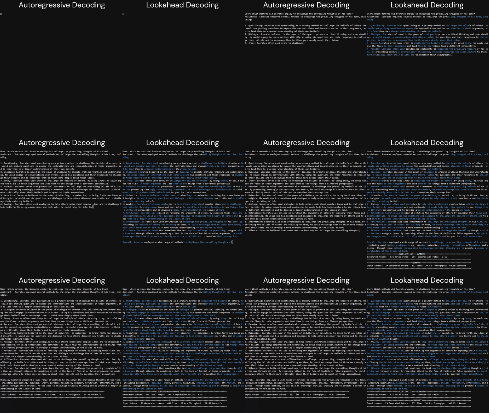
Figure 1: Demo of speedups by lookahead decoding on LLaMA-2-Chat 7B generation. Blue fonts are tokens generated in parallel in a decoding step.
Introduction
Large language models (LLMs) like GPT-4 and LLaMA are rapidly reinventing today's applications, but their inference -- based on autoregressive decoding -- is very slow and difficult to optimize. Each autoregressive decoding step generates only one token at a time; as a result, the latency of an LLM request primarily depends on the response length of the request or, equivalently, the number of decoding steps. Making matters worse, each decoding step does not leverage the parallel processing power of modern GPUs, often resulting in low GPU utilization. This challenges many real-world LLM applications that prioritize rapid response time, such as chatbots and personal assistants, which frequently generate long sequences with low latency.
One way to accelerate autoregressive decoding is speculative decoding (including Medusa and OSD), which employ a "guess-and-verify" strategy: a draft model predicts several potential future tokens, and the original LLM then verifies these guesses in parallel. These approaches can opportunistically reduce the number of decoding steps and, consequently, lower latency. However, they face several limitations. First, the maximum speedup that speculative decoding based methods can achieve is limited by the token acceptance rate, or equivalently, how accurately the draft model can predict the main model's outputs. Second, creating an accurate draft model is non-trivial, often requiring extra training and careful tuning in the face of traffic changes over time.
In this blog post, we introduce a new, exact decoding algorithm, lookahead decoding, designed to overcome these challenges. The key observation enabling lookahead decoding is that, although decoding multiple next tokens in one step is infeasible, an LLM can indeed generate multiple disjoint n-grams in parallel. These n-grams could potentially fit into future parts of the generated sequence. This is achieved by viewing autoregressive decoding as solving nonlinear equations and adapting the classic Jacobi iteration method for parallel decoding. The generated n-grams are captured and later verified, if suitable, integrated into the sequence.
Lookahead decoding is able to generate n-grams each step, as opposed to producing just one token, hence reducing the total number of decoding steps -- generating N tokens in less than N steps. In fact, lookahead decoding stands out because it:
- Operates without a draft model, streamlining deployment.
- Linearly reduces the number of decoding steps relative to log(FLOPs) per step.
Next, we will show that lookahead decoding provides a substantial reduction of latency, ranging from 1.5x to 2.3x with negligible computation overhead. More importantly, it allows one to trade computation for latency reduction, albeit this comes with diminishing returns.
We have developed an implementation of lookahead decoding compatible with huggingface/transformers. Users can easily enhance the performance of HuggingFace's native generate function with just a few lines of code. We encourage you to explore our code repository and provide feedback.
Background: Parallel LLM Decoding Using Jacobi Iteration
The Jacobi iteration method is a classic solver for non-linear systems. In the case of LLM inference, we can also employ it for parallel token generation without a draft model. To see this, let's reconsider the autoregressive decoding process. Traditionally, this process is seen as a sequential generation of tokens, illustrated in Figure 2(Left). With some simple rearrangements of equations, it can be conceptualized as solving a system of non-linear equations, as depicted in Figure 2(Right).
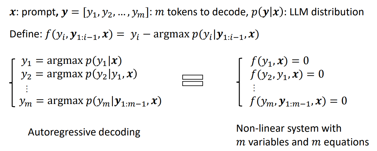
Figure 2: Autoregressive decoding as a process of solving non-linear systems.
An alternative approach based on Jacobi iteration can solve all of this nonlinear system in parallel as follows:
- Start with an initial guess for all variables .
- Calculate new values for each equation with the previous .
- Update to the newly calculated .
- Repeat this process until a certain stopping condition is achieved (e.g., ).
We illustrate this parallel decoding process (also referred to as Jacobi decoding) in Figure 3. Jacobi decoding can guarantee solving all variables in at most steps (i.e., the same number of steps as autoregressive decoding) because each step guarantees at least the very first token is correctly decoded. Sometimes, multiple tokens might converge in a single iteration, potentially reducing the overall number of decoding steps. For example, as shown in Figure 3, Jacobi decoding predicts and accepts two tokens, "computer" and "scientist," in a single step (Step 4).
Compared to autoregressive decoding, each Jacobi decoding step is slightly more expensive in terms of FLOPs needed because it requires LLM forward computation on >1 token. Fortunately, this usually does not translate into slowdowns, thanks to the parallel processing nature of GPUs.
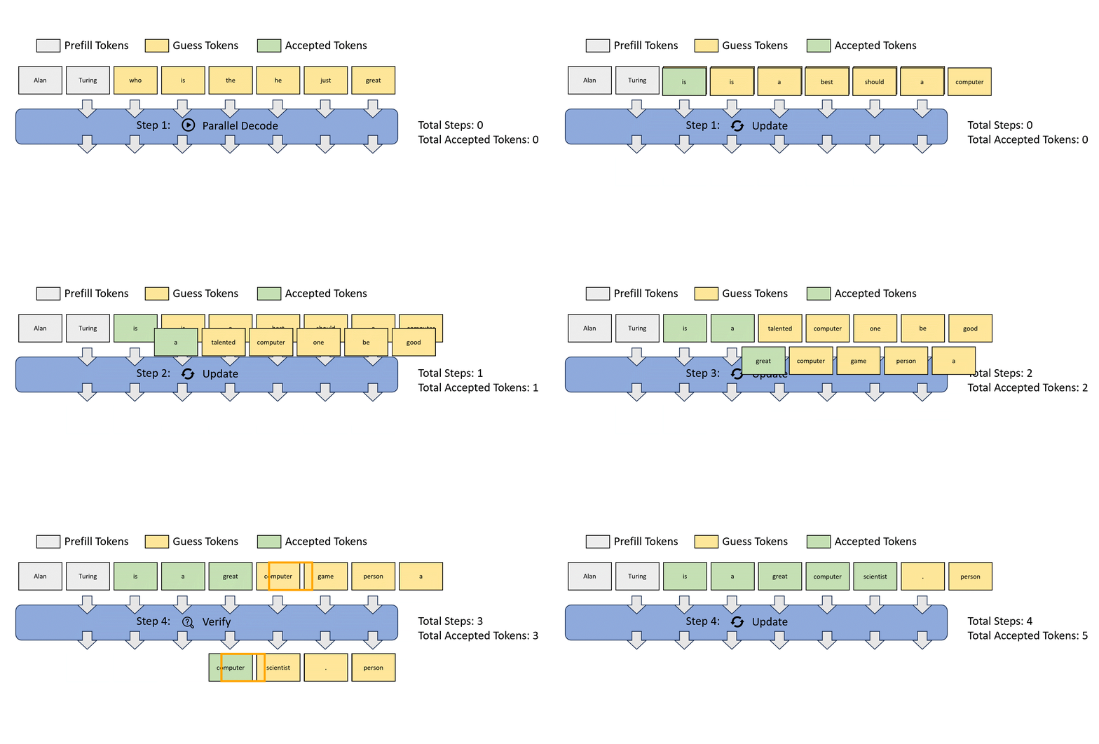
Figure 3: Illustration of applying Jacobi iteration method for parallel LLM decoding.
Limitations of Jacobi Decoding
In practical applications, we have found that Jacobi decoding faces several challenges that impede achieving considerable wallclock speedup. While it can decode more than one token in many steps, precisely positioning these tokens within the sequence often goes wrong. Even when tokens are correctly predicted, they are often replaced in subsequent iterations. Consequently, very few iterations successfully achieve the simultaneous decoding and correct positioning of multiple tokens. This defeats the fundamental goal of parallel decoding.
Lookahead Decoding
Lookahead decoding overcomes the limitations of Jacobi Decoding by leveraging its capability of generating parallel n-grams. In Jacobi decoding, we notice that each new token at a position is decoded based on its historical values from previous iterations. This process creates a trajectory of historical tokens at each token position, forming many n-grams. For instance, by looking back over three Jacobi iterations, a 3-gram can be formed at each token position. Lookahead decoding takes advantage of this by collecting and caching these n-grams from their trajectories. While lookahead decoding performs parallel decoding using Jacobi iterations for future tokens, it also concurrently verifies promising n-grams from the cache. Accepting an N-gram allows us to advance N tokens in one step, significantly accelerating the decoding process. Figure 4 illustrates this process.
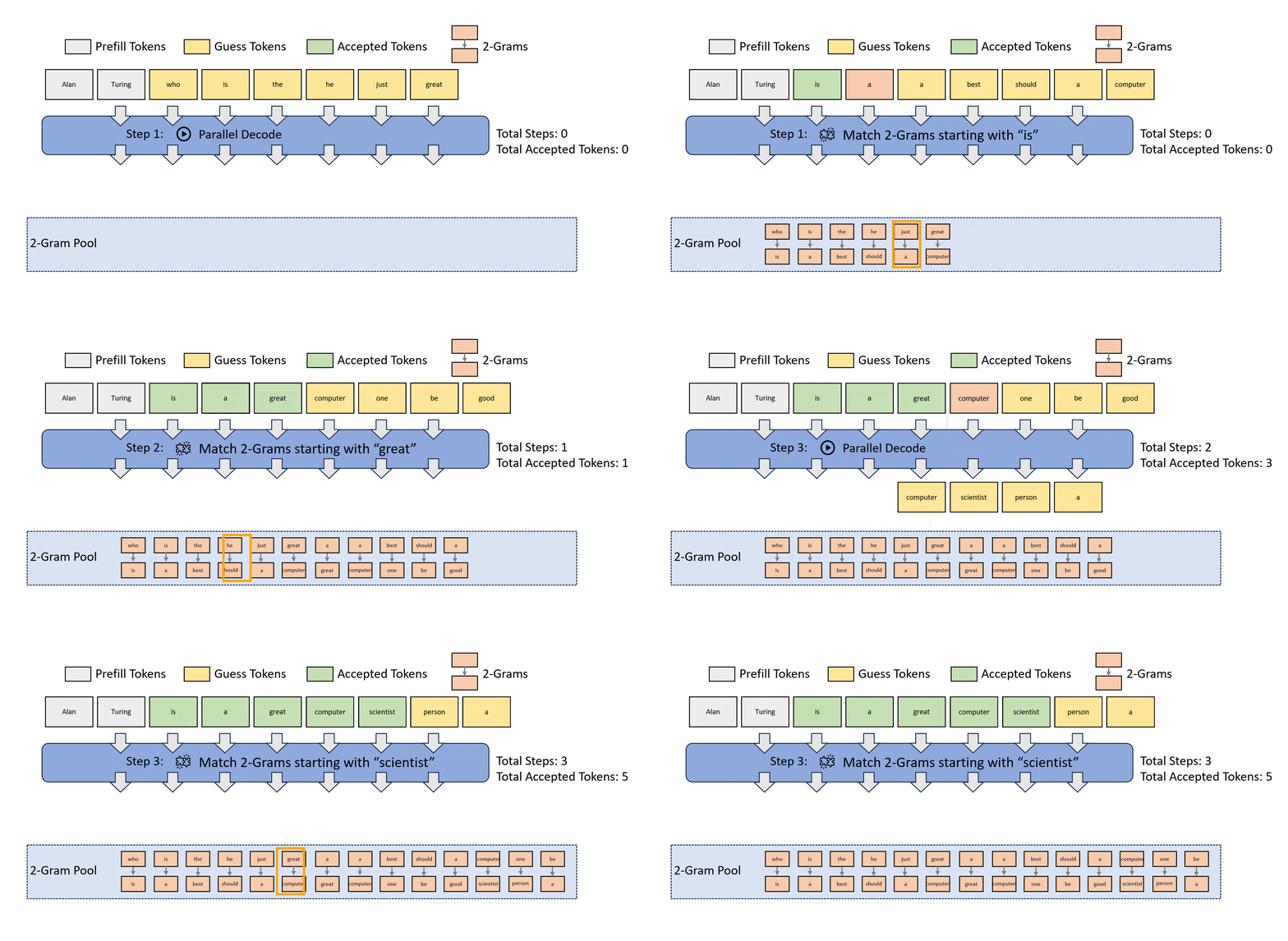
Figure 4: Illustration of lookahead decoding with 2-gram.
To enhance the efficiency of this process, each lookahead decoding step is divided into two parallel branches: the lookahead branch and the verification branch. The lookahead branch maintains a fixed-sized, 2D window to generate n-grams from the Jacobi iteration trajectory. Simultaneously, the verification branch selects and verifies promising n-gram candidates.
Lookahead Branch
The lookahead branch aims to generate new N-grams. The branch operates with a two-dimensional window defined by two parameters:
- window size : how far ahead we look in future token positions to conduct parallel decoding.
- N-gram size : how many steps we look back into the past Jacobi iteration trajectory to retrieve n-grams.
Consider Figure 5 as an illustrative example. Here, we look back at 4 steps () in the trajectory and look ahead at 5 tokens () for future positions. In the figure, the blue token labeled 0 is the current input. The tokens in orange, green, and red were generated in previous Jacobi iterations at steps , , , respectively. The number on each token indicates its position relative to the current input token (the blue one marked with 0). At the current step , we conduct one Jacobi iteration to generate new tokens for all 5 positions, using the trajectory formed by the previous 3 steps. Then, we collect 4-grams -- for example, a 4-gram could comprise the orange token at position 1, the green token at position 2, the red token at position 3, and the newly generated token at the current step.
As the decoding progresses, tokens from the earliest step in the trajectory are removed to maintain the defined and parameters. It's important to note that when , lookahead decoding essentially becomes equivalent to Jacobi decoding.
Verification Branch
Alongside the lookahead branch, the verification branch of each decoding step aims to identify and confirm promising n-grams, ensuring the progression of the decoding process. In the verification branch, we identify n-grams whose first token matches the last input token. This is determined via a simple string match. Once identified, these n-grams are appended to the current input and subjected to verification via an LLM forward pass through them. As the n-gram cache grows, it becomes increasingly common to find multiple n-grams that start with the same token, which raises the verification cost. To manage the cost, we set a cap of on the number of candidate n-grams considered in the verification branch. In practice, we often set this cap proportional to (e.g., ).
Lookahead and Verify In The Same Step
Since LLM decoding is primarily bounded by memory bandwidth, we can merge the lookahead and verification branches in the same step, leveraging GPU's parallel processing power to hide overheads. This is achieved by designing a special attention mask shown in Figure 5, which adheres to two rules: (1) The tokens in the lookahead branch cannot see tokens in the verification branch, and vice versa. (2) Each token only sees its preceding tokens and itself as in a casual mask. We have implemented the attention mask in HuggingFace. We are in the process of developing a more efficient custom CUDA kernel to speed up the execution further.
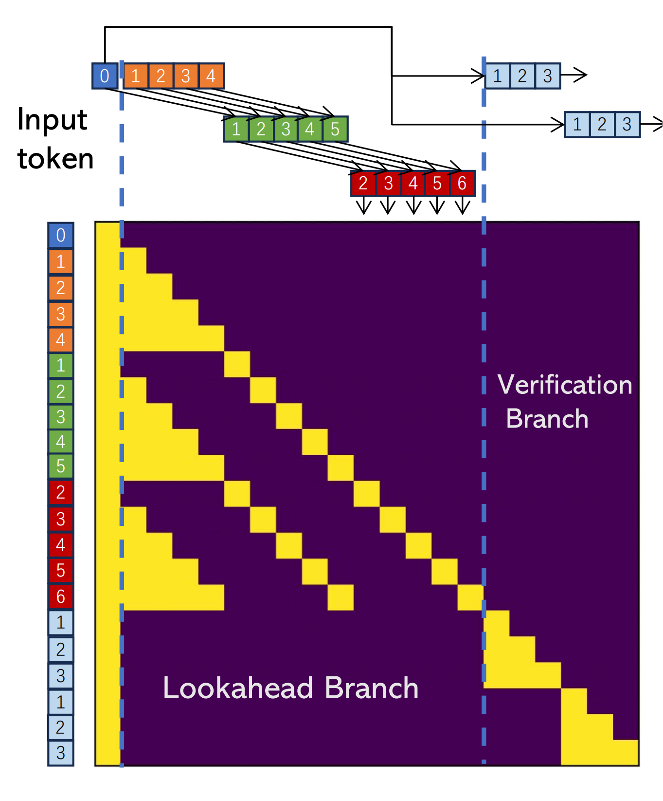
Figure 5: Attention mask for lookahead decoding with 4-grams and window size 5. In this mask, two 4-gram candidates (bottom right) are verified concurrently with parallel decoding.
Scaling Law of Lookahead Decoding
Lookahead decoding can generate different N-grams and verify candidates per step. As (the lookahead window size) and (the N-gram size) increases, so do the computational operations per step. However, this increase also enhances the likelihood of accepting a longer n-gram with a step. In other words, lookahead decoding allows to trade more flops for reducing latency, provided the system is not constrained by computational capacity.
To examine the scaling behavior of lookahead decoding, we analyze the number of decoding steps required for a given number of tokens, varying the values of and . The findings are illustrated in Figure 6. Notably, when the n-gram size is sufficiently large (e.g., ), exponentially increasing the future token guesses (window size ) can linearly reduce the number of decoding steps. We refer to this phenomenon as the scaling law of lookahead decoding.
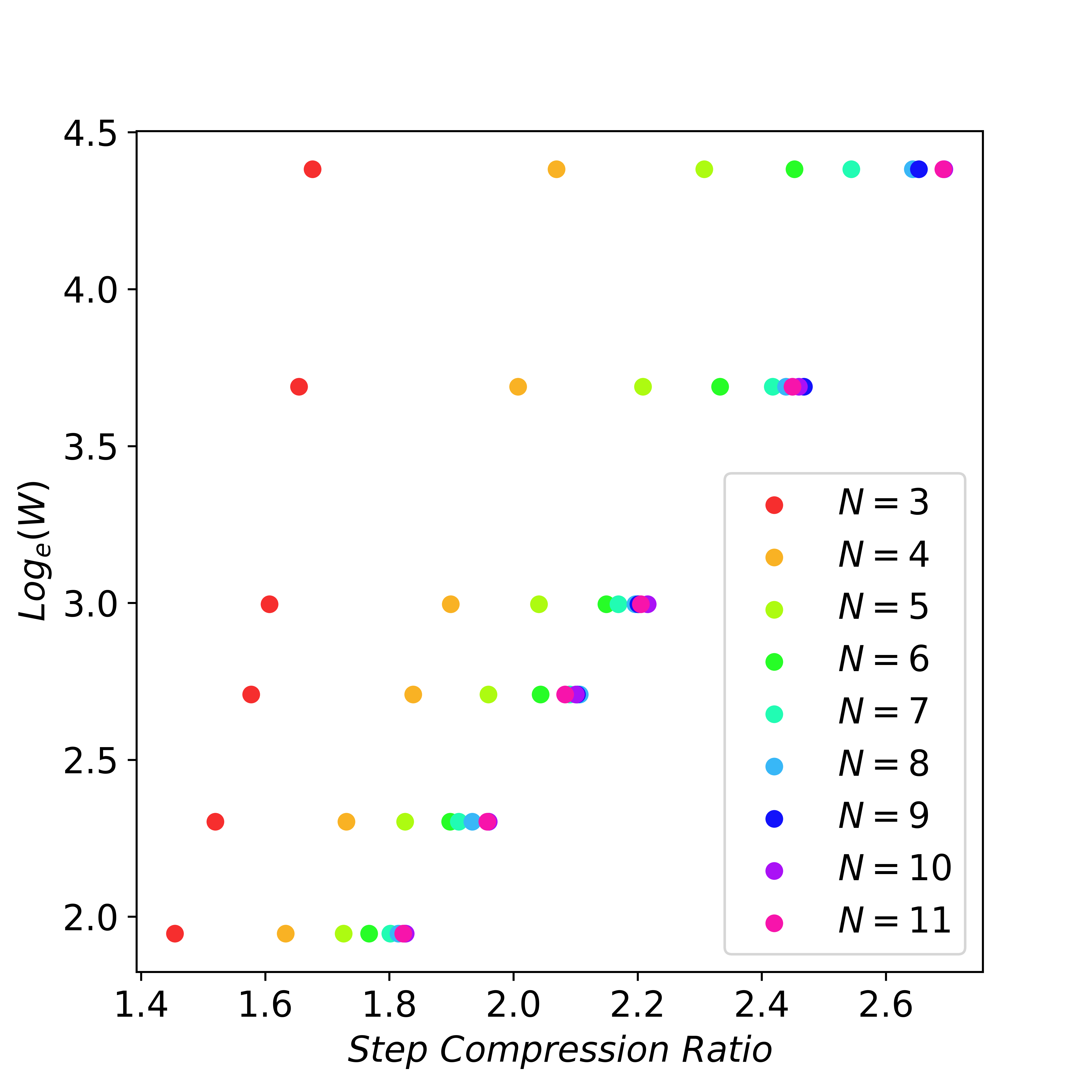
Figure 6: When $N$ is large enough, exponentially increasing window size $W$ can linearly reduce the number of decoding steps. Here we set $G=W$. Experiments are conducted using LLaMA-2-chat 7B on MT-Bench dataset.
Cost, Usage, and Limitations
The FLOPs needed for each lookahead decoding step are proportional to the number of input tokens per step, which is the sum of the lookahead branch size and the verification branch size: . As the scaling law reveals, when is large enough, an exponential increase in the can result in a linear reduction of decoding steps. Thus, we can achieve linear compression of the steps by trading exponentially more FLOPs since we set .
Given this property, lookahead decoding should be used in scenarios where latency is vital, e.g., surplus FLOPs exist that can be traded for latency, or it is even worthwhile to pay extra FLOPs for latency. For powerful GPUs (e.g., A100), lookahead decoding can better squeeze its performance by using a large and to achieve low latency when generating long sequences. However, if and are too large, each lookahead decoding step might be too costly and slow down the decoding despite reducing decoding steps. Increasing together with would be best to achieve balanced performance, avoiding hitting a theoretical cap if only increasing one side. Our experimental results show that on A100, the following configs in Table 1 work well in most cases. The 7B, 13B, and 33B models require 120x, 80x, and 56x extra FLOPs per step, respectively. However, because of the memory-intensive bound characteristic of the LLM decoding, these extra FLOPs only bring little per-step cost and a visible step compression ratio, resulting in a notable speedup.
Table 1. Good configurations for window size W and N-gram size N on A100.
| Model | Window Size ($W$) | N-gram Size ($N$) |
| 7B | 15 | 5 |
| 13B | 10 | 5 |
| 33B | 7 | 5 |
You can also change the setting to tune a better performance on your specific decoding latency requirement.
Experimental Result
We evaluate the efficiency of lookahead decoding on LLaMA-2-Chat and CodeLLaMA of various sizes on different datasets including MT-bench, HumanEval, and GSM8K. Note that lookahead decoding achieves speedup without any finetuning or draft models. The 7B, 13B, and 33B models are evaluated on a single A100 GPU, and the 70B model is evaluated on two A100 GPUs with pipeline parallelism, all under fp16 precision.

Figure 7: Speedup of lookahead decoding on different models and datasets.
LLaMA-Chat on MT-Bench. Lookahead decoding achieves roughly 1.5x speedup across several model settings.
CodeLLaMA on HumanEval. Applying lookahead decoding to CodeLLaMA on HumanEval shows more than 2x latency reduction. This is because many repeated N-grams are present in code which can be correctly guessed.
CodeLLaMA-Instruct on GSM8K. Using CodeLLama-Instruct to solve math problems from GSM8K, lookahead decoding achieves a 1.8x latency reduction.
Get Started with Lookahead Decoding
We have implemented lookahead decoding in huggingface's transformers. You can accelerate your transformers' decoding API with only a few LoCs. Please check our GitHub repo and give us feedback!
Acknowledgment
We would like to thank Richard Liaw, Yang Song, and Lianmin Zheng for providing insightful feedback.
Citation
@misc{fu2023lookahead,
    title = {Breaking the Sequential Dependency of LLM Inference Using Lookahead Decoding},
    url = {https://lmsys.org/blog/2023-11-21-lookahead-decoding/},
    author = {Yichao Fu and Peter Bailis and Ion Stoica and Hao Zhang},
    month = {November},
    year = {2023}
}